Geometric Brownian Motion: Simulating Price Paths — Shown Through SPY

Geometric Brownian Motion (GBM) is the canonical continuous-time model for asset prices. It powers the Black–Scholes framework, Monte-Carlo risk engines, and most of the intuition practitioners carry about “what could the price do?”.

1.Summary

GBM assumes that percentage returns — not price changes — are random, normally distributed, and independent over time. Prices therefore stay positive and their terminal distribution is log-normal. Two parameters fully describe the model: the drift $μ$ (expected annual log-growth plus half-variance) and the volatility $σ$ (annualised standard deviation of log returns) — both estimable directly from historical data.

2.Intuition

2.1Returns compound, prices don't add

A $10 move means something very different at SPY = 100 than at SPY = 600. What is comparable across price levels is the relative move. GBM makes randomness proportional to the current price: $dS = μS dt + σS dW$ .

2.2Why log-normal

If each day multiplies the price by a small random gross return, the log-price is a sum of many small independent shocks — and sums of independent shocks are (approximately) normal. Normal log-price $\Rightarrow$ log-normal price: skewed right, floored at zero.

2.3Drift vs. noise

Over short horizons the noise term dominates ( $σ t$ shrinks slower than $μt$ as $t \to 0$ ); over long horizons drift wins. This is the same $t$ rule that governs plain Brownian motion — GBM simply wraps it in an exponential.

3.Theory & Mechanics

3.1The SDE and its solution

d S_{t} = μ S_{t} dt + σ S_{t} d W_{t}

Applying Itô’s lemma to $l n S_{t}$ (the $- \frac{1}{2} σ^{2}$ correction comes from $(dW)^{2} = dt$ ):

S_{t} = S_{0} e x p [(μ - \frac{1}{2} σ^{2}) t + σ W_{t}]

3.2Exact discretisation

Because the solution is closed-form, we can simulate without discretisation error at any step size $Δ t$ :

S_{t + Δ t} = S_{t} \cdot e x p [(μ - \frac{1}{2} σ^{2}) Δ t + σ Δ t Z], Z \sim N (0, 1)

Two small functions implement this: one draws per-step gross returns, the other compounds them into price paths.

python

def gbm_returns(mu, sigma, dt, n_steps, n_paths):
    """One-step gross returns under GBM (shape: n_steps x n_paths)."""
    z = np.random.normal(size=(n_steps, n_paths))
    return np.exp((mu - 0.5 * sigma**2) * dt + sigma * np.sqrt(dt) * z)

def gbm_paths(s0, mu, sigma, dt, n_steps, n_paths):
    """Price paths of shape (n_steps + 1, n_paths), starting at s0."""
    rets = gbm_returns(mu, sigma, dt, n_steps, n_paths)
    return s0 * np.vstack([np.ones(rets.shape[1]), rets]).cumprod(axis=0)

4.Applied Example — SPY

4.1Calibrate $μ$ and $σ$ from real data

We pull daily SPY prices, estimate annualised drift and volatility from log returns, and let the data — not guesses — drive the simulation.

python

TICKER = "SPY"
START, END = "2018-01-01", "2024-12-31"

def load_prices(ticker, start, end):
    """Adjusted-close prices: yfinance first, Stooq as fallback."""
    try:
        import yfinance as yf
        df = yf.download(ticker, start=start, end=end, auto_adjust=True, progress=False)
        if not df.empty:
            return df["Close"].squeeze().rename(ticker).dropna()
    except Exception as exc:
        print(f"yfinance failed ({exc}); trying Stooq…")
    url = f"https://stooq.com/q/d/l/?s={ticker.lower()}.us&i=d"
    df = pd.read_csv(url, parse_dates=["Date"], index_col="Date")
    return df.loc[start:end, "Close"].rename(ticker).dropna()

px = load_prices(TICKER, START, END)
log_ret = np.log(px / px.shift(1)).dropna()

s0        = float(px.iloc[-1])
sigma_hat = float(log_ret.std() * np.sqrt(252))
mu_hat    = float(log_ret.mean() * 252 + 0.5 * sigma_hat**2)  # drift of the SDE, not of log returns

print(f"{TICKER}: {len(px)} daily observations, last close = {s0:,.2f}")
print(f"mu_hat    = {mu_hat:.2%}  (annualised drift)")
print(f"sigma_hat = {sigma_hat:.2%}  (annualised volatility)")

4.2Simulate 1,000 five-year paths

Grey lines are individual paths, the dashed line is the mean of the simulated distribution, and the band spans the 5th–95th percentile — the “cone of plausible futures”.

python

DT      = 1 / 252
HORIZON = 252 * 5          # 5 years
N_PATHS = 1_000

paths = gbm_paths(s0, mu_hat, sigma_hat, DT, HORIZON, N_PATHS)
t_ax  = np.arange(paths.shape[0]) / 252

p5, p95 = np.percentile(paths, [5, 95], axis=1)

fig, ax = plt.subplots(figsize=(10, 5))
ax.plot(t_ax, paths, color="gray", lw=0.2, alpha=0.35)
ax.fill_between(t_ax, p5, p95, color="steelblue", alpha=0.25, label="5–95% band")
ax.plot(t_ax, paths.mean(axis=1), "k--", label="Mean path")
ax.set_title(f"{TICKER}: {N_PATHS:,} GBM paths, 5 years  (mu={mu_hat:.1%}, sigma={sigma_hat:.1%})")
ax.set_xlabel("Years"); ax.set_ylabel("Simulated price"); ax.legend()
plt.tight_layout(); plt.show()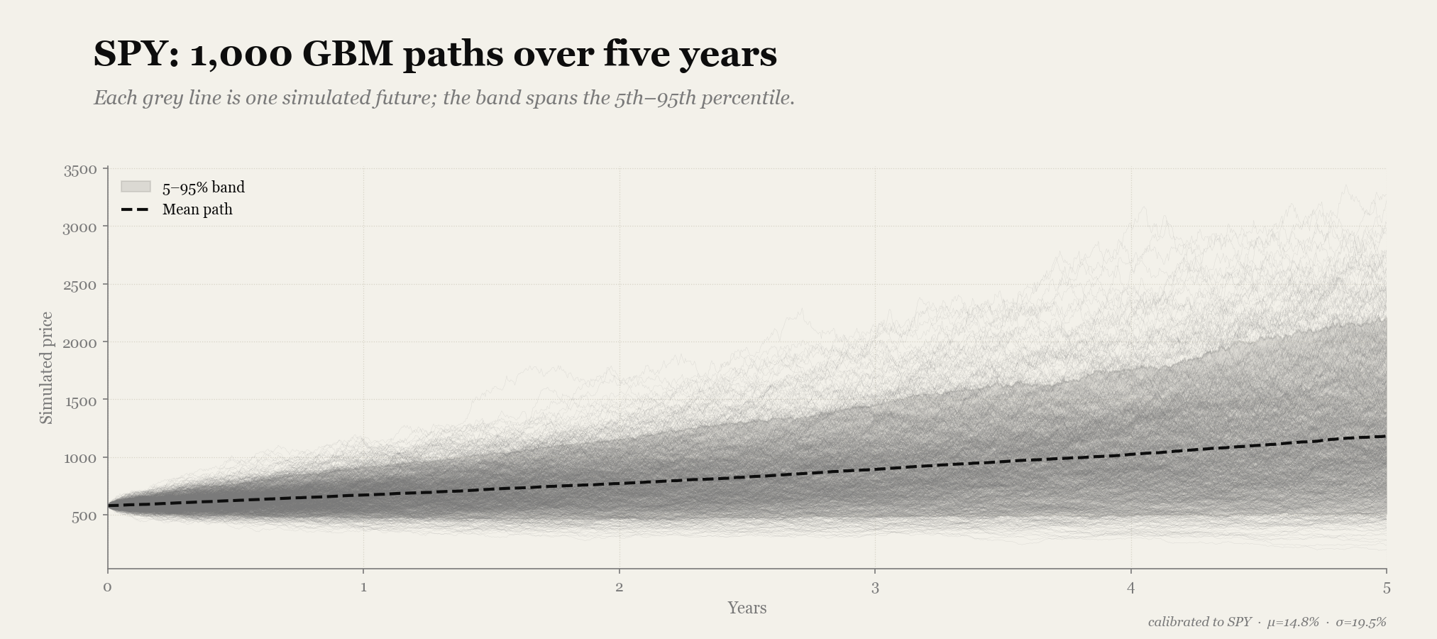

One thousand simulated SPY price paths fanning out over five years; a shaded band spans the 5th to 95th percentile and a dashed line marks the mean path — Figure 4.2 · SPY — 1,000 GBM paths over five years

4.3Terminal distribution — is it log-normal?

Theory says $l n S_{T} \sim N ((μ - \frac{1}{2} σ^{2}) T, σ^{2} T)$ . Overlaying the theoretical density on the simulated histogram is a one-line correctness check — and shows the characteristic right skew: the mean sits above the median.

python

from scipy import stats

T   = HORIZON / 252
s_T = paths[-1]

x   = np.linspace(s_T.min(), s_T.max(), 400)
pdf = stats.lognorm.pdf(x, s=sigma_hat*np.sqrt(T),
                        scale=s0*np.exp((mu_hat - 0.5*sigma_hat**2)*T))

fig, ax = plt.subplots(figsize=(10, 4))
ax.hist(s_T, bins=60, density=True, color="steelblue", alpha=0.55, label="Simulated $S_T$")
ax.plot(x, pdf, "k-", lw=1.5, label="Theoretical log-normal")
ax.axvline(s_T.mean(),   color="black", ls="--", label=f"Mean   {s_T.mean():,.0f}")
ax.axvline(np.median(s_T), color="red",  ls="--", label=f"Median {np.median(s_T):,.0f}")
ax.set_title(f"{TICKER}: terminal price distribution after {T:.0f} years")
ax.set_xlabel("Price"); ax.legend()
plt.tight_layout(); plt.show()

Histogram of simulated terminal SPY prices with the theoretical log-normal density overlaid; dashed lines mark the mean above the median, showing the right skew — Figure 4.3 · SPY — terminal price distribution after five years

4.4Sanity check: switch the drift off

With $μ = 0$ , GBM is a martingale: the mean terminal price must sit at $S_{0}$ . A quick way to catch implementation bugs (a common one: forgetting the $- \frac{1}{2} σ^{2}$ correction, which inflates the mean).

python

paths_nd = gbm_paths(s0, 0.0, sigma_hat, DT, HORIZON, N_PATHS)
print(f"Mean terminal price (no drift): {paths_nd[-1].mean():,.2f}   vs   S0 = {s0:,.2f}")

5.Conclusion

5aStrengths

Analytically tractable — closed-form solutions (Black–Scholes) make it the natural baseline
Positive prices, log-normal terminal distribution — matches the basic stylised fact that prices can't go negative
Only two parameters — both estimable directly from historical log returns
Cheap to simulate — vectorised NumPy generates millions of paths in seconds

5bWeaknesses & Limitations

Constant volatility — real vol clusters and spikes
No jumps — crashes like March 2020 are far outside its reach
Normal log-returns — real returns have fat tails
Independent increments — momentum and mean-reversion exist

5cApplications in Practice

Baseline for option pricing and Monte-Carlo risk engines
Scenario cones for wealth projections
Null model against which fancier models must justify their complexity

5dAlternatives & Extensions

Stochastic volatility — Heston (see our Quant Insights piece “Heston vs Black-Scholes: fitting the volatility smile”)
Jump-diffusion — Merton
GARCH-family models — for clustered volatility

Geometric Brownian Motion: Simulating Price Paths — Shown Through SPY

1.Summary

2.Intuition

2.1Returns compound, prices don't add

2.2Why log-normal

2.3Drift vs. noise

3.Theory & Mechanics

3.1The SDE and its solution

3.2Exact discretisation

4.Applied Example — SPY

4.1Calibrate μ and σ from real data

4.2Simulate 1,000 five-year paths

4.3Terminal distribution — is it log-normal?

4.4Sanity check: switch the drift off

5.Conclusion

5aStrengths

5bWeaknesses & Limitations

5cApplications in Practice

5dAlternatives & Extensions

4.1Calibrate $μ$ and $σ$ from real data